


 |
Maple, in conjunction with MapleSim and the MapleSim Control Design Toolbox, provides extensive capabilities for plant modeling and advanced control system design. Maplesoft tools provide you with the ability to:
- Rapidly develop complex, high-fidelity plant models in an intuitive multi-domain modeling.
- Characterize all possible solutions to a given control problem and then pick the best solution based on the particular situaton.
- Build and investigate controllers where the model includes symbolic, unspecified parameters. The same controller design can then be applied to multiple related models without further tuning.
- Create controllers where the design specifications are parametric, so the same controller can be used successfully under a variety of conditions.
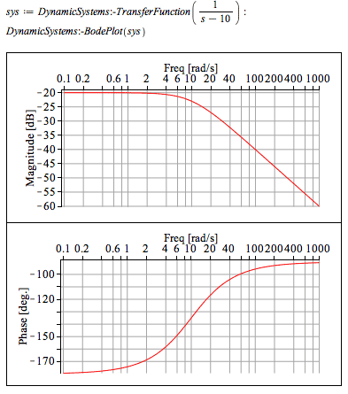
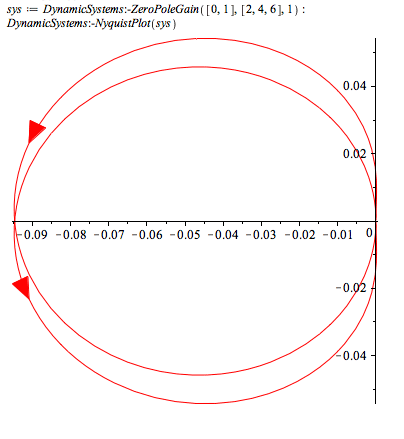
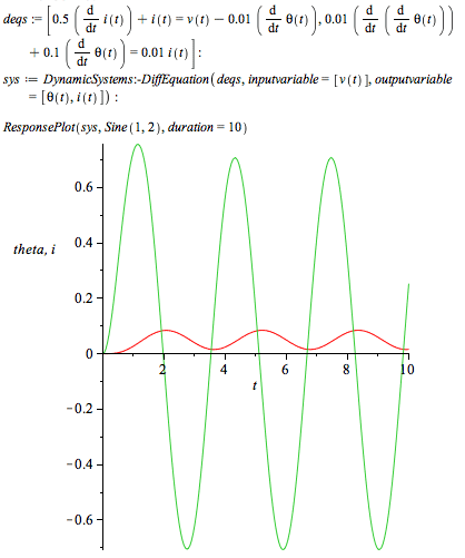
- Define your linear and nonlinear systems using one of four different representations: differential equations, transfer functions, state-space matrices, or zero-pole-gain. Maple allows you to convert between these representations both programmatically or through the context-sensitive menu.
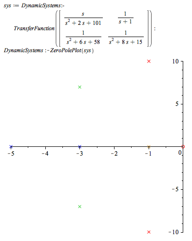
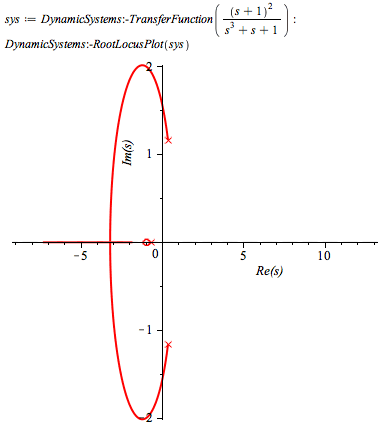
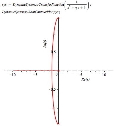
- Analyze your system using a variety of standard analysis tools from Bode, Nyquist, Zero Pole, Nichols, Root Locus, and Root Contour plots to observability, controllability, and Routh tables.
- Compute the operating points for your system and linearize your model around those operating points.
- Implement the Ziegler-Nichols (time and frequency response) as well as Cohen-Coon PID tuning strategies.
- Take advantage of advanced PID tuning methods such as dominant pole placement, pole placement in a specified region, and gain and phase margin.
- Develop state-feedback controllers such as LQR, single input pole placement (using Ackermann's formula) and multiple input pole placement
- Apply state estimation techniques such as Kalman filters, single output pole placement (using Ackermann's formula) and multiple output pole placement.
Navigate to:
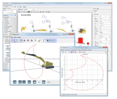
Maplesoft's suite of tools for modeling and analyzing engineering systems provides a wide range of capabilities for advanced control system design. The tight integration that exists between Maple, MapleSim, and the MapleSim Control Design Toolbox gives engineers the ability to create detailed plant models and the analytical tools for controller development and testing. Moreover, the symbolic computation engine that lies at the core of these tools provides you with greater flexibility and accuracy in your control systems design. With these tools, engineers can dramatically reduce the time and cost of up-front analysis, virtual prototyping, and parameter optimization of their system designs.
Model Linearization
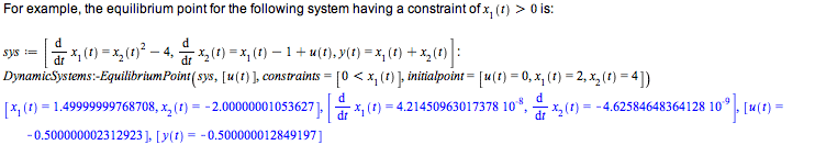
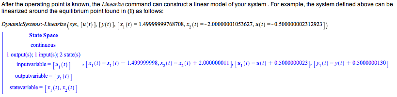
Using the EquilibriumPoint command, Maple gives you the ability determine the local equilibrium point of your system satisfying constraints. The command performs a local search and returns an equilibrium point closest to the initial point, either specified by the initialpoint parameter or chosen randomly. If the EquilibriumPoint command cannot find a point at which derivatives are zero, it returns a point that minimizes the derivatives. It is possible to prescribe a nonzero value to the derivatives using the optional parameter constraints.
Control Design Algorithms
Maple, in conjunction with MapleSim and the MapleSim Control Design Toolbox, provides you with numerous algorithms for control design. The following list provides you with an overview of Maple's capabilities in the area of standard PID tuning, advanced PID tuning, state feedback control and state estimation.
Standard PID and Advanced PID Tuning:
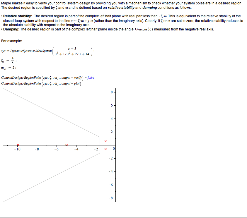
- Characterize all PID controllers for pole placement in a desired region.
- PID tuning based on the Cohen-Coon method
- PID controller design for (dominant) pole placement
- Find feasible controller gains for pole placement in a desired region.
- PID tuning based on gain and phase margin specifications
- Ziegler-Nichols frequency domain (closed-loop) identification
- Identify parameters of a first-order with time-delay (FOTD) model using time domain techniques.
- PID tuning based on Ziegler-Nichols frequency domain (closed-loop) methods
- PID tuning based on Ziegler-Nichols time domain (open-loop) methods
State Feedback Control:
- Design linear quadratic state feedback regulator (LQR) for a given state space.
- Design continuous-time linear quadratic state feedback regulator (LQR) for a given pair.
- Design discrete-time linear quadratic state feedback regulator (LQR) for a given pair .
- Design linear quadratic state feedback regulator (LQR) with output weighting.
- Calculate the state feedback gain for single-input systems using Ackermann's formula.
- Calculate the state feedback gain for single-input or multiple-input systems.
State Estimation:
- Design Kalman estimator for a given state space.
- Calculate the observer gain for single-output systems using Ackermann's formula.
- Construct the static-gain (Luenberger) observer for given observer gain.
- Calculate the observer gain for single-output or multiple-output systems.
Example: Pole Placement Method

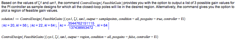
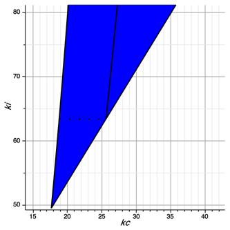
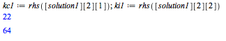
For this example, we will use the gain values for kc and ki as provided above:
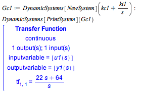
Using these gain values, the transfer function for the PI controller can be determined as:
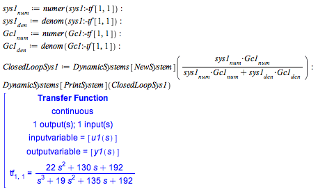
At this point, we can obtain the transfer function for the closed-loop system.
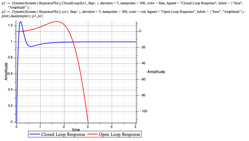
The step response of the open and closed-loop system can be determined using the DynamicSysetms[ResponsePlot] command. From the plots, we can see how the including of a PI controller was able to stabilize the system.
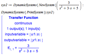
Example: Exact Pole Placement Method
In this section, we will show how the exact pole placement method is used to design a PID controller for a 2nd order system. As in the previous section, the transfer function of the open loop system can be defined as follows:
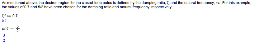
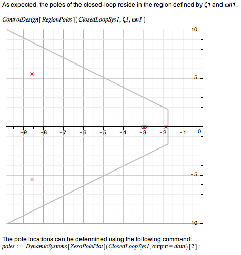
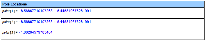
Let's assume that the desired closed-loop pole locations are:
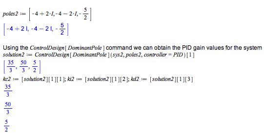
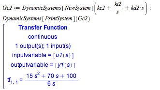
Using these gain values, the transfer function for the PID controller can be determined:
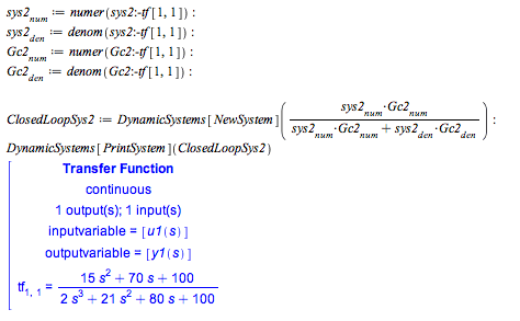
At this point, we can obtain the transfer function for the closed-loop system.
The step response of the open and closed-loop system is shown in the following plots. The closed-loop response in addition to tracking the input signal is much faster than then open-loop response.
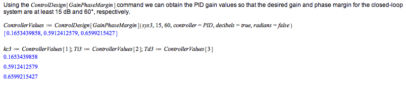
Example: Gain-Phase Margin Method
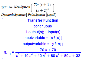
In this section, we will show how the gain-phase margin method is used to design a PID controller for the following fifth-order system.
The system gain margin (in decibels) and associated crossover frequency (in rad/sec) is:
![]()
Similarly, the system phase margin (in degrees) and crossover frequency (in rad/sec) is:
![]()
Using these gain values, the transfer function for the PID controller can be determined as:
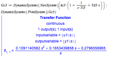
At this point, we can obtain the transfer function for the closed-loop system.
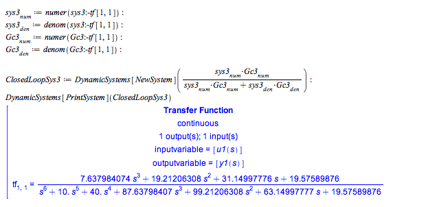
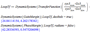
The gain and phase margin and crossover frequencies for the loop transfer function are shown below. These values exceed the minimum requirements specified above.
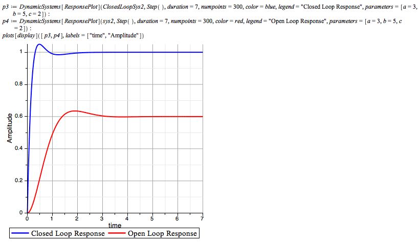
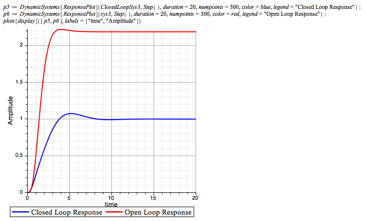
The step response of the open and closed-loop system is shown in the following plots. Unlike the open-loop response which was more than 100% off in the steady state, the closed-loop response now tracks the input signal.
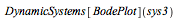
The bode plots of the open-loop system and the loop transfer function are shown below.

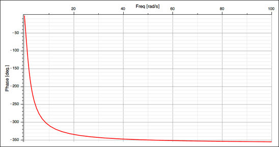
![]()
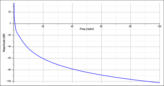
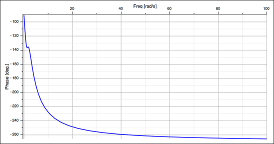
![]()
System Definition and Analysis
Maple provides you with several options to define your system. Choose between a frequency-based representation or a time-based representation:
| Frequency-Based Representation | Time-Based Representation |
| Transfer function model | State-space model |
| Zero-pole-gain model | Differential equation model |
| Coefficient model | Algebraic equation model |
In addition, Maple makes it easy to define and analyze your plant and controller models. The following list outlines Maple's capabilities in this area:
- Compute the characteristic polynomial of a state-space system.
- Compute the controllability matrix.
- Determine controllability of a state-space system.
- Compute the gain-margin and phase-crossover frequency.
- Compute the controllability and observability grammians.
- Compute the observability matrix.
- Determine observability of a state-space system.
- Return the phase-margin and gain-crossover frequency.
- Generate the Routh table of a polynomial.
- Reduce a state-space system.
- Perform similarity transformations on state-space matrices.
- Compute the properties of a step response.
- Determine equivalent system representation of two or more interconnected system objects.